Convert Pivot Tables with Power Query to Import into Power BI
TABLEAU / POWERBI


Are you a data enthusiast who's just getting started with Power BI? If you've been working with pivot tables in Excel and want to leverage the powerful capabilities of Power BI for data visualization and analysis, you're in the right place. In this beginner's guide, we'll walk you through the process of converting a pivot table into a format suitable for importing into Power BI. Let's dive in!
Let's say you just got in your hands an excel pivot table and want to import into Power BI.
The problem?
You need to trasnform it in a way the table is more suitable for visualization.
Don't worry, we'll walk you through step by step to make it more useful in Power BI.
Step 1: Prepare Your Pivot Table
Before we begin, make sure you have an Excel workbook with a well-organized pivot table. Ensure that the table contains clear headers, meaningful data, and minimal formatting. Clean up any unnecessary rows or columns that won't be part of your analysis.
If you want to follow this practice exercise, access pivot table HERE.
Step 2: Load Data into Power BI
Open Power BI Desktop, the software where you'll create your data visualizations.
From the "HOME" tab, select "GET DATA."
Choose "Excel" as your data source and locate the Excel file containing your transformed table.
Click "Import" to proceed.
Step 3: Transform Data in Power Query Editor
Power Query Editor is a powerful tool within Power BI that allows you to clean, shape, and transform your data before using it in your visualizations.
Once you've imported your data, Power Query Editor will open automatically.
Here, you can apply various transformations to your data. This might involve removing redundant columns, merging tables, renaming columns, or applying filters.
For our example table, let’s transform a few things:
Remove top 2 NULL rows in Power Query
Select first row, go to top ribbon, and click on ‘REMOVE TOP ROWS’
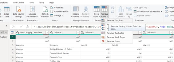
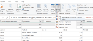
Since we want to remove the first 2 rows, lets specify it as 2 number of rows since they are useless for our data visualization.
If you like this content and want to learn more, you might also read:
Essential Technical Skills for Data Analysts
Power BI with SQL for Beginners
Power BI: Data Insights for Smarted Decisions
The Power of Data Visualization Tools: A Visual Journey through Insights
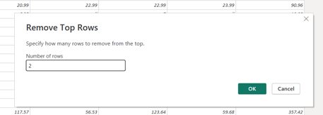
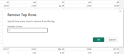
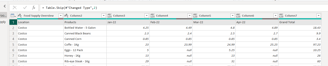
After clicking OK, rows will be removed.
Change columns headers in Power Query
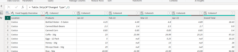
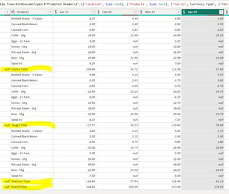
When we look at the data, we see location, products, months, and grand total as the first row. But we actually want it as columns name.
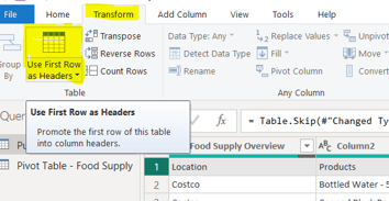
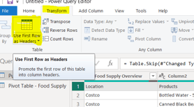
Go to top ribbon in ‘TRANSFORM’, then ‘USE FIRST ROW AS HEADERS’.
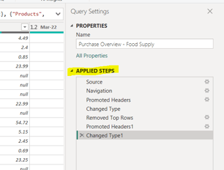
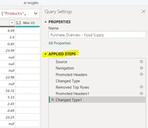
If for some reason you made a mistake and want to change it, just go to ‘APPLIED STEPS’ and remove the step you want to go back.
Now, we have them as our headers.
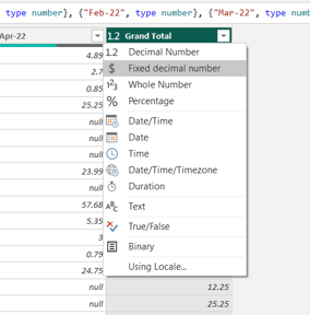
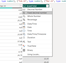
Change data type in Power Query
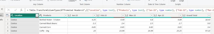
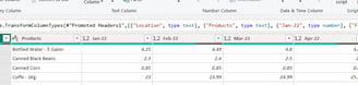
As right now, our columns are ‘DECIMAL NUMBERS’, however, we want it to be ‘FIXED DECIMAL NUMBER’ ($).
Click on ‘1.2’, which represents the data type of the column, and chose the right type for the column. In this case, ‘FIXED DECIMAL NUMBER’ ($).
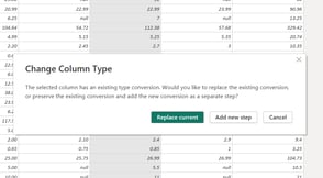
Select ‘REPLACE CURRENT’.

Do it for all columns with ($) values.
Remove unwanted rows in Power Query
In this case, let's remove store's total rows.
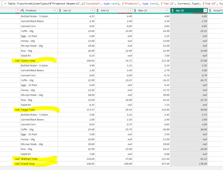
Since we do not need these rows for our visualization, let’s remove them by removing empty in ‘LOCATION’ column.
Click on the drop-down arrow, and ‘REMOVE EMPTY’.
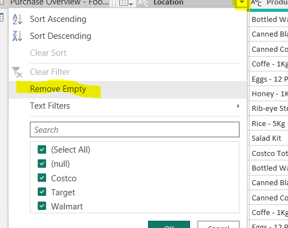
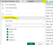
As result, we have a table with no NULL rows.
Another option to filter out NULL rows is go to drop-drown, ‘TEXT FILTERS’, ‘DOES NOT CONTAIN’…
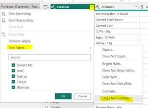
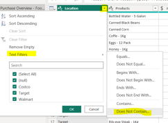
Then, specify ‘Total’ as they are NULL.
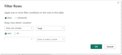
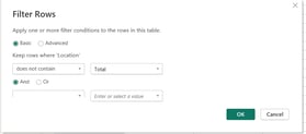
---- Just giving you a couple of options to bring the same result.
Remove unwanted columns in Power Query
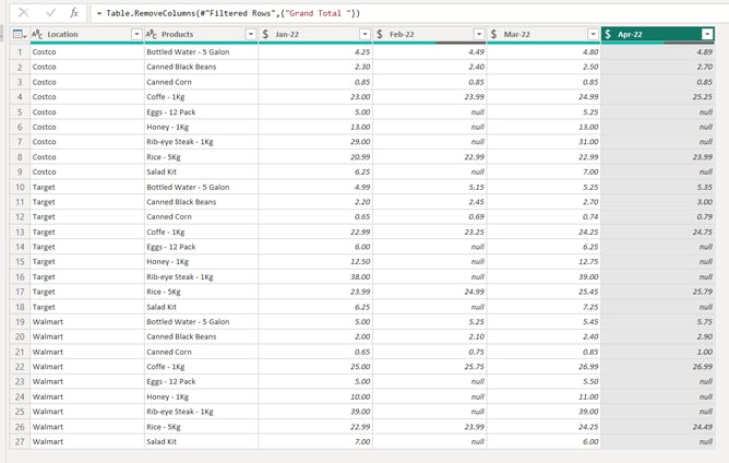
Since we can perform all calculations in POWERBI, let’s remove GRAND TOTAL column as we do not need it.
Click on the column header to select it, ‘HOME’, ‘REMOVE COLUMNS’.
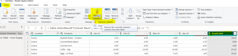
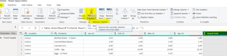
Note: If it opens a window saying ‘INSERT’, it’s because it’s inserting into ‘APPLIED STEPS’.
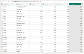
Here is how our table is looking like:
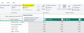
Transpose / Unpivot columns in Power Query
When it comes to visualization, columns with dates do note really work. To fix it, let’s transpose or pivot so dates are actually rows.
Let’s select all 4 columns, ‘TRANSFORM’ tab, ‘UNPIVOT COLUMNS’.
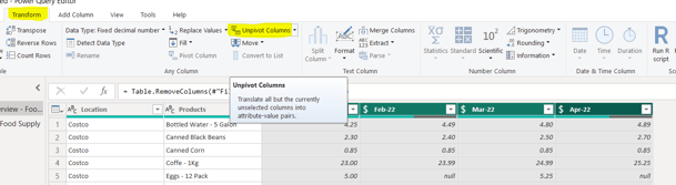
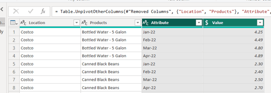
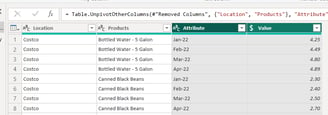
Now, our table is in right format that is much suitable for visualization.
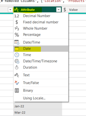
Final clean up
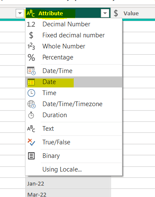
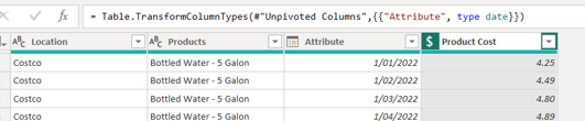
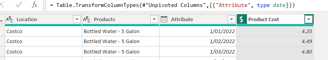
Let’s change ‘ATTRIBUTE’ data type as date.
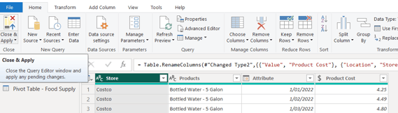
And let’s rename ‘VALUE’ column as ‘PRODUCT COST’ by double clicking on it.
And let’s change ‘LOCATION’ to ‘STORE’ by double clicking as well.
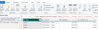
Step 4: Load Transformed Data into Power BI
After you've completed your data transformations, click the "Close & Apply" button in Power Query Editor.
Power BI will load your cleaned and transformed data into its data model, where you can build compelling visualizations.
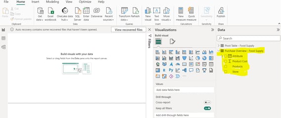
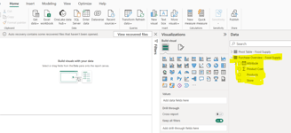
Step 5: Build Visualizations and Reports
With your data loaded, you can start creating visualizations. Power BI offers a wide range of visualization options, including charts, graphs, tables, and more.
Drag and drop fields from your data model into the visualization panes to create meaningful reports.
Step 6: Share and Collaborate
Once you've created your visualizations and reports, you can save your Power BI project.
Power BI offers options for sharing your reports with others. You can publish your reports to the Power BI service, where colleagues or stakeholders can view them.
Congratulations!
You've successfully converted a pivot table from Excel into a format suitable for importing into Power BI. By following these steps, you can harness the full potential of Power BI to create insightful visualizations and reports that help you make data-driven decisions. Remember that practice makes perfect, so don't hesitate to experiment and explore all the features Power BI has to offer.
Start your journey into the world of data analysis and visualization with Power BI today and unlock a new level of data-driven insights!